
In aquaculture breeding systems, genetic gain is usually achieved through a dedicated breeding nucleus composed of a relatively small number of elite animals. However, from a commercial perspective, it is the realised genetic gain in production animals that is important. The efficiency with which genetic gain is transmitted from the nucleus to production varies considerably between species, groups and with the design and operation of the breeding program. This post examines the nature of genetic transmission losses and what can be done to minimise them, using examples from fish and shrimp production systems.
The basics
The breeding population needs to contain sufficient genetic diversity to manage inbreeding and enable trait improvement through selection. The pace of genetic gain (DGnucleus) is a function of both the selection intensity and the accuracy of selection. The selection process itself was described in a previous post. Briefly, the genetic merit of selection candidates is inferred from accurate measurements of their phenotypes (or that of close relatives) and are expressed as a breeding value (EBV).
Variations in DNA sequence influencing the trait are called alleles. Alleles that act independently of other alleles or the environment can be simply summed up to find their contribution to the trait – this is the so-called additive genetic effects that are represented by the EBVs. There is another kind of genetic variation which has non-linear effects and is therefore non-additive. It includes dominance where one allele contributes the effect of two alleles of the same type, or epistasis where the effect of one allele depends on the presence of other alleles, or gene-environment (G x E) interactions where the contribution of an allele varies with the environment in which the animal is farmed.
Additive genetic variation is inherited predictably from parents to offspring, whereas non-additive genetic variation is not, because dominance and epistasis depend on specific allele combinations that may not be conserved across generations. These types of non-additive genetic variation serve to reduce within‑family variance and may overestimate the genetic merit of some families, changing the ranking of selection candidates. Fortunately, non-additive genetic effects are generally modest for many traits but can be significant for survival and disease resistance traits.
Genetic transmission losses
Some of the genetic gain expected from nucleus crosses fails to materialise in production animals because of transmission losses. The realised response in genetic gain (DG) observed in production animals can be expressed by a simple equation:

where each multiplier represents a specific transmission constraint. T represents the genetic correlation between nucleus breeders and production animals and varies with genetic connectedness, number of multiplication steps and the control of family contributions. C represents the conversion of genetic merit through reproduction and captures unequal representation of families due to skewed mating success, high early mortality of elite families and inbreeding depression. E represents expression efficiency in the production environment and is the genetic correlation between nucleus testing and production environments. Strong G x E interactions will serve to reduce the genetic correlation between the nucleus and farm.
Maximising genetic gain on the farm
To achieve the best possible performance in production animals, it is necessary to maximise genetic improvement in the breeding nucleus whilst genetic transmission losses. Some important considerations for achieving these twin objectives are considered below.
1. Maintain a large effective population size in the breeding nucleus
A large effective population size in terms of numbers of genetically distinct families and individuals per family results in a high standing genetic variation and provides the scope for effective inbreeding control (reduces C) and applying a high selection intensity (proportional to DGnucleus). What large exactly means in practice depends on the species being farmed and the scale of production.
2. Implement genomic selection and choose the “best” genetic prediction model
Genomic selection (GS) is the preferred method for calculating EBVs in modern breeding programmes. Typically, 50 – 70K genome-wide SNP markers are used to predict Genomic Estimated Breeding Values (GEBVs). This involves genotyping and phenotyping a training population comprising an equal weighting of the offspring from the families represented in the nucleus to develop the genomic prediction model. The selection candidates held in the nucleus only need to be genotyped. The “best” prediction model is the one with the highest accuracy for the target trait (proportional to DGnucleus).
Linear mixed models such as GBLUP use a genomic relationship matrix and assume many alleles with small, additive effects. They are simple to implement and interpret, robust, and show high prediction accuracies for traits with a range of heritability values (Table 1). Single step GBLUP allows animals to be included that only have pedigree (rather than genomic) information to increase prediction accuracy.
Trait | Phenotype definition | Heritability | Prediction accuracy |
Juvenile body weight | 0.60 | 0.70 | |
Lice count after challenge | 0.21 | 0.65 | |
Survival vs death after pancreas disease challenge | 0.42 | 0.78 |
Table 1: GBLUP prediction accuracies for traits in Atlantic salmon. The examples have strong statistical support. Prediction accuracy is reported as the correlation between true and predicted breeding values, estimated via cross‑validation.
Models that can handle G x E interactions reduce genetic transmission losses due to E. Such effects are unimportant when the nucleus testing environment is similar to that of production environments. However, when they are different, a failure to consider G x E effects can result in a reranking of selection candidates and environment-specific genetic effects which reduce the realised genetic gain.
The negative impacts of G x E on prediction accuracy are particularly severe in shrimp breeding programmes because the biosecure nucleus environment is very different from that of the shallow ponds used for grow-out which are characterised by highly variable temperatures, salinities and pathogen pressures. As a rule of thumb when genetic correlation between environments is below 0.8, ignoring G x E leads to reduced genetic gain.
There are two main methods for including G x E effects in GBLUP prediction models. Multi-environment GBLUP (ME-GBLUP) involves measuring the same trait in different environments and makes use of the genetic correlation between environments to quantify G x E. For shrimp the genetic correlations between growth in the biosecure nucleus and farm ponds can be less than 0.5 in some circumstances. Simulation studies found ME_GBLUP to be effective in offsetting genetic losses from G x E, albeit at the expense of significantly increased genotyping costs.
The other approach is to model breeding values as a function of a continuous environmental gradient to capture plasticity and robustness. This so-called reaction-norm (RN) method was used to analyse growth of Atlantic salmon in Tasmania over 14 summers and 2 sites with average temperatures varying from 12.8 – 19.7oC. Heat tolerance was assessed in terms of a standardise heat load. The prediction accuracy with ssGBLUP was 0.55 for highest heat load and 0.53 for thermal sensitivity – derived from the slope of the reaction norm. This looks like a promising method to improve the resilience of Atlantic salmon to future ocean warming. The rise of precision aquaculture involving the continuous and automatic collection of environmental data from multiple sensors for temperature, salinity and oxygen across all production sites provides a ready source of data for such reaction norm models of genomic selection.
Several other classes of genetic prediction model are available. Bayesian prediction models don’t assume all SNPs have an equal effect and can outperform GBLUP when a few relatively strong alleles explain most of the genetic variation. The downside of Bayesian models is that they are computationally intensive, harder to tune and interpret and still largely only capture additive effects. Machine learning (ML) models make fewer biological assumptions and learn complex relationships directly from data. ML models naturally capture dominance, epistasis, non-linear effects and some G x E effects. They can also readily incorporate digital image data such as body shape. However, for most traits prediction accuracies are often comparable to GBLUP and Bayesian models. A disadvantage of ML models is that they require much larger training sets (>5,000 animals) which significantly increases genotyping costs. ML models are also computationally intensive, tend to be unstable, come with the risk of over fitting and most importantly of all their internally workings are something of a mystery providing little or no biological insight.
The take home message is that no single model is “best” under all circumstances. GBLUP is usually a good choice for growth and performs well for most traits such that it has become the standard model used in most breeding programmes. For complex, non-linear traits where dominance, epistasis and G x E are very important Bayesian and ML models may give superior prediction accuracy but at a cost. The optimal strategy is probably to use GBLUP as a baseline and to use ML models selectively for the most complex non-linear traits.
3. Instigate effective inbreeding control
Optimum Contribution Selection is a method of fixing co-ancestry at a predefined level to maximise genetic gain whilst controlling inbreeding levels in the next generation (reduces C). Specialist software such as Optimate uses evolutionary algorithms that mimic biological evolution to test all possible mating scenarios against each other to deliver the best possible genetic gain while keeping inbreeding at the desired level. Some software is so efficient that it provides mating solutions in almost real time. This enables preprepared mating plans to be modified on the day of striping according to the availability of mature animals – a very useful feature in a busy hatchery.
4. Optimise the breeding scheme to minimise genetic transmission losses
Genetic transmission losses vary with the breeding scheme and reproductive biology of the species being farmed.
Atlantic Salmon
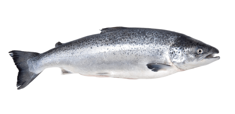
Salmo salar
The genetic correlation between nucleus and production is high and genetic transmission losses correspondingly modest when eyed ova from the nucleus are directly sourced for production. The conversion of genetic merit through reproduction benefits from targeted crosses, high hatching success of eggs and low mortality rates of juvenile stages. Genetic gain is highest when training populations and selection candidates are composed of families of equal size. Realised genetic gain is significantly reduced if multiplier broodstock are added to the breeding scheme because mass selection and uncontrolled matings serve to weaken the genetic correlation between nucleus and production animals. Improvements in nucleus performance are also delayed by a generation interval when multipliers are used.
White-leg shrimp
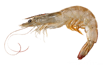
Litopenaeus vannamei
Shrimp are bred from Specific Pathogen Free (SPF) broodstock held in high-biosecurity facilities and then progressively multiplied and disseminated through multiplication centres, hatcheries and grow-out farms. Genetic transmission losses are low in the nucleus but occur at each successive stage. Multiplication centres convert elite genetics into a large number of breeders. The number of animals increases dramatically but because of weak mating control and unbalanced and low larval survival (<20%) genetic transmission losses are significant. The net result is reduced effective population size, genetic drift, loss of family representation and implicit selection for robustness unrelated to selection traits. Multiplication should be viewed as a dissemination not a selection step. Culling based on hatchery traits should therefore be avoided. Transmission losses would be reduced by more structured mating e.g., breeding within smaller groups of mature individuals and by achieving more equal representation of nucleus families. Ultra-low density SNP panels may provide sufficient family assignment accuracy at a price point which makes selective genotyping of multipliers an attractive commercial proposition.
Hatcheries produce post larvae (PLs) for sale using mass spawning which further weakens the genetic correlation between the nucleus and farm causing more transmission losses. Finally, the realised genetic gain in grow-out farms is reduced by G x E, disease and density effects. A meta-analysis quantified how much of the genetic gain achieved in nucleus environments fails to transmit to shrimp farms based on data from the literature. The mean genetic correlation for growth traits between breeding and farm environments was around 0.72. Thus, if the nucleus achieves a 10% per‑generation gain in body weight, less than three quarters was expressed on farms. Because of stronger G x E effects only about 60% of the nucleus genetic gain for survival was realised on farms. These results emphasise the importance of considering G x E in the genomic prediction model and adjusting the breeding scheme to minimise genetic transmission losses.
Final thoughts
This post has highlighted the importance of focusing on the realised responses to selection. It is important to track realised gain in production animals and to adjust the program when nucleus gains are not being satisfactorily transmitted. Investment in reducing transmission losses may prove as or more profitable than incremental nucleus gains achieved through ever more sophisticated genomic selection models.
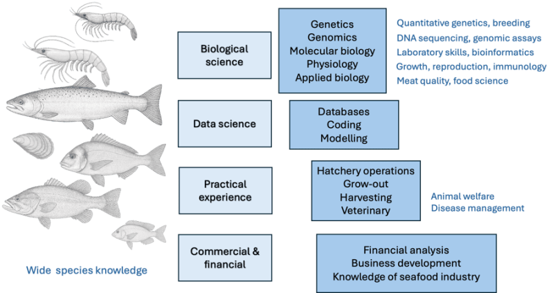
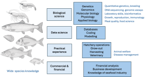
Fig. 1 Skills and expertise needed to successfully audit and manage a modern aquaculture breeding programme.
All the options to maximise genetic gain discussed come with some incremental infrastructure and/or operational costs. Best practice requires an ongoing analysis of the benefit-cost ratio for each intervention to achieve the best commercial return on investment. The audit and management of a modern aquaculture breeding programme is no easy task without the right resources (Fig. 1). Fortunately, specialist genetics and breeding companies have built the experienced multidisciplinary scientific teams and advanced software needed to efficiently manage the genetic complexities of breeding programmes and associated bioeconomic modelling. These companies also have the advantage of scale across their customer base enabling them to offer high-density genotyping at highly competitive low prices per sample.
This article concludes our Insights with Ian series, where we have explored key principles shaping modern aquaculture breeding programmes.